Part 48 Text Data
48.1 Wrangling
We’ve been working primarily with numerical-based data. However, we might also be interested in text-based data. This field of study is called Natural Language Processing (NLP).
Keeping in scope with the class being “How do we wrangle/program with our data?” we will go over how to wrangle and shape text-based data as well as some metrics to measure important words.
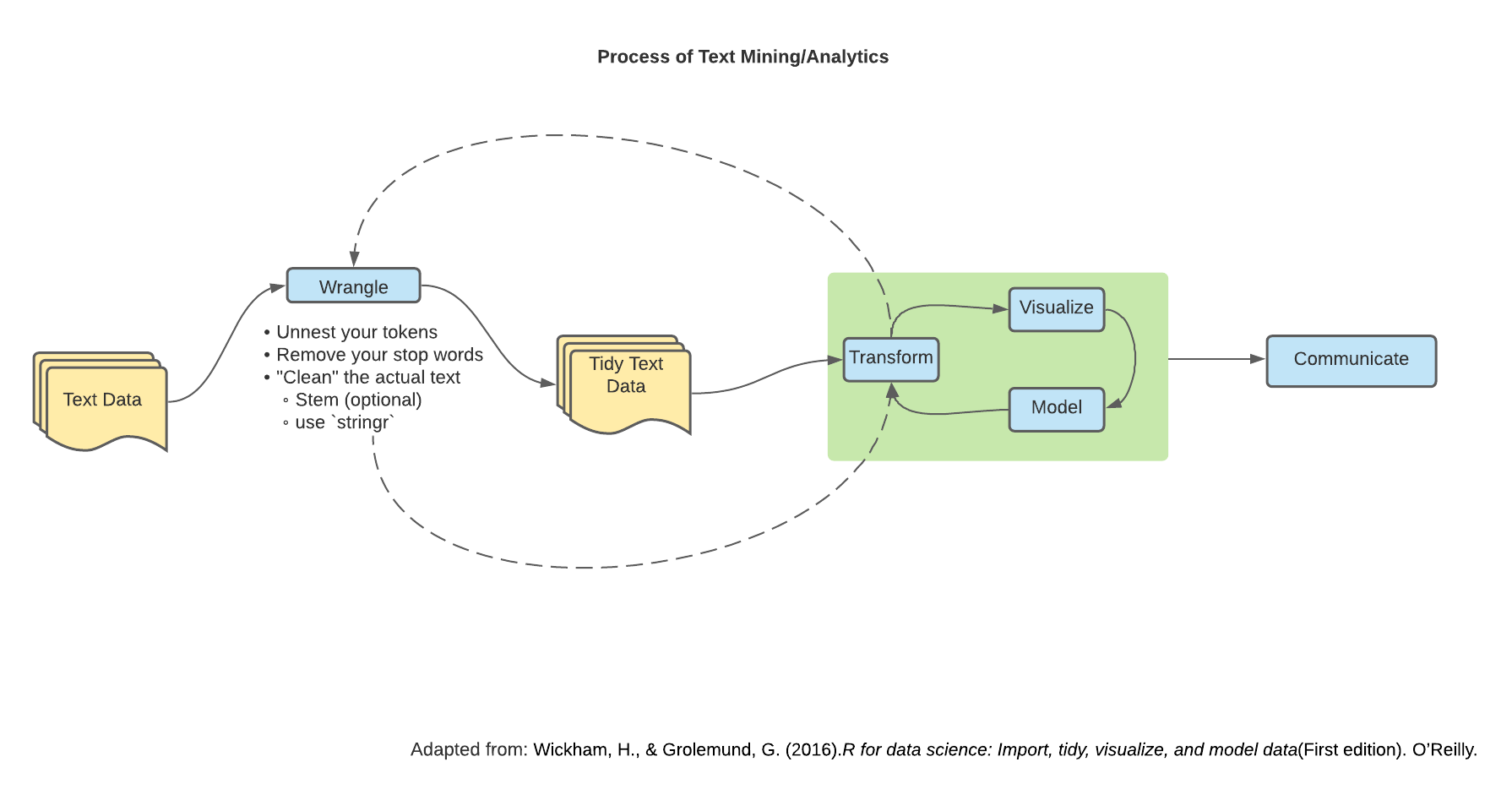
The primary package we will be using to wrangling is the tidytext package.
Another useful package for text (or string) manipulation is the stringr package.
48.2 Natural Language Processing (NLP) - Terminology
In your journey of NLP, you might stumble across different terms used and it’s important to get familiar with them so we can start formulating our ideas and expressing our questions with the terminology.
Corpus - A broad collection of documents
- Plural: Corpora
Document - A collection of terms
Terms - Words
Tokens - The unit of the analysis (words, characters, sentence, paragraph, n-grams, etc.)
- Changes meaning based off what we are wanting to analyze
- We tokenize our data; the process of splitting text into tokens
Read more about other key terms here.
48.3 The mighty unnest_tokens() function
Lets look at an example of some text:
text <- c("Today and only today is a lovely day to learn about text data and NLP",
          "I hope that one day I will be able to apply all of what I learn because learning if cool and fun",
          "If I were to express my feelings in two words: excitement and anxious")

text
Now let’s put it into a data frame structure:
text_df <- tibble(
  line = 1:3,
  text = text
)

text_df
48.4 Tidy data text principles
The “tidy data” principles apply to text data as well!
We want our data to have one-token-per-document-per-row. In our case, tokens are individual words.
The main three arguments of unnest_tokens() look like this:
unnest_tokens(data_frame, new_name_of_column, column_name_in_data_frame)or
data_frame |>
  unnest_tokens(new_name_of_column, column_name_in_data_frame)
Let’s take a look at what that looks like:
unnest_df <-
  text_df |>
  unnest_tokens(word, text)

unnest_df
I’m sure you’ve noted a few things about our text from using unnest_tokens()
Our words are split into a word-per-row
We have a way of identifying from which document (
line) our words come fromOur words are…lower case?
48.5 Clean your text! Grammar vs. Computers
In English (and broadly all language), we have grammar. Computers don’t. This has big implications.
We need to make sure that we capture our words (or tokens) as we understand them. Computers don’t know that “Capital Word” is the same thing as “capital word”. They also don’t know that “running” is the same idea as “run”.
I’m sure you already have thought of practical solutions to some of these problems and guess what? We do exactly that.
48.6 Capitalization
This one’s pretty easy: we make all our text the same format. Usually lowercase is the format of choice. I like lowercase because then I’m not being yelled at.
unnest_tokens() automatically makes words lowercase. We can change that by specifying to_lower = FALSE. (In the case we are working with URLs.)
48.7 Stemming
For words that have the same “stem” (or root) we can remove the end.
Example:
These words:
Consult
Consultant
Consultants
Consulting
Consultative
Become:
- Consult
We can specify this in unnest_tokens() with token = argument. Look at ?unnext_tokens() to see the different types of tokens the function offers.
These grammar vs. computer problems don’t stop here (nor do their solutions).
48.8 Regular Expressions (Regex) for URLS
Depending on the text data we are working with, we might either be interested (or not interested) in URLs. Using regular expressions, we can try and detect URLs within our text. Regular expressions are a whole other beast so to keep in scope with the class, here is one example of a regular expression for URLs with a little explanation.
(http|https)([^\\s]*)The
(http|https)looks for “http” or “http” at the start of a string.The
([^\\s]*)means “keep matching until a white space”
Using stringr we can select different str_* functions to aid in our goal.
Here are a list of texts that have a URL in different places within the string.
url_front <- c("https://regex101.com/ is an awesome website to check out different regular expressions")
url_middle <- c("One of my friends suggested I look at https://www.youtube.com/watch?v=dQw4w9WgXcQ for a good tutorial on regular expressions")
url_back <- c("Here is a good resource on regex: https://stackoverflow.com/questions/tagged/regex")

urls <- c(url_front, url_middle, url_back)
We can create functions to help us do it!
remove_url <- function(text) {
  # Regex
  url_regex_expression <- "(http|https)([^\\s]*)"

  # Removes URL
  text <- stringr::str_remove(
    string = text,
    pattern = url_regex_expression
  )

  return(text)
}

extract_url <- function(text) {
  # Regex
  url_regex_expression <- "(http|https)([^\\s]*)"

  # Extracts URL
  text <- stringr::str_extract(
    string = text,
    pattern = url_regex_expression
  )

  return(text)
}
Putting it all together can call the function either on each individual string…
# Individual URL matching
remove_url(url_middle)
extract_url(url_middle)
…or within a list like so:
# Group URL matching
remove_url(urls)
extract_url(urls)
48.9 Counting words
Now that we have our tidy text data frame, we can start digging in.
Let’s add a count of each word:
unnest_df |>
  count(word, sort = TRUE)
But lets work within our sentences (or documents)
count_df <-
  unnest_df |>
  group_by(line) |>
  count(word, sort = TRUE)
count_df
Lets look at a (not) very interesting graph of what we have:
library(ggplot2)

count_df |>
  ggplot() +
  aes(y = n, x = forcats::fct_reorder(word, n, max)) + # sort our bars
  geom_col() +
  coord_flip() + # flip the coords (easier to digest graph)
  facet_wrap(~ line, scales = "free_y") + # let our y axis be free
  labs(y = "word",
       x = "count")
From the graph above, we can see that we have a lot of words that don’t really carry a lot of meaning.
48.10 Can’t stop (words) won’t stop (words)
Not all words are created equal - some words are more important than others. Words like “the”, “a”, “it” don’t have any inherent meaning. Pronouns also may not be meaningful “he”, “their”, “hers”. These are called stop words
So what do we do? Get rid of ’em.
How? We get a stop words data set and anti_join() them. There exists many stop word data sets. These are sometimes called “Lexicons”. You can think of a lexicon as a set of words with a common idea.
48.11 Lexicon-based approach
Some common (and native) stop word data sets (or Lexicons) are:
Onix
SMART
snowball
These are all within the tidytext package’s stop_words data set.
This is a glimpse of what it looks like:
tidytext::stop_words |>
  head()
Now let’s remove our stop words.
unnest_df <-
  count_df |>
  anti_join(stop_words, by = "word")
Here we can see our words with substance.
unnest_df |>
  ggplot() +
  aes(x = word, y = n) +
  geom_col() +
  facet_wrap(~ line, scale = "free_y") +
  coord_flip()