Part 20 The pipe advantage
20.1 Learning Objectives
By the end of this lesson, you will:
- Have a sense of why dplyr is advantageous compared to the “base R” way with respect to good coding practice.
Why?
- Having this in the back of your mind will help you identify qualities of and produce a readable analysis.
20.2 Compare nested functions to pipe chains
Self-documenting code.
This is where the tidyverse shines.
Example of dplyr vs base R:
gapminder[gapminder$country == "Cambodia", c("year", "lifeExp")]vs.
gapminder |>
  filter(country == "Cambodia") |>
  select(year, lifeExp)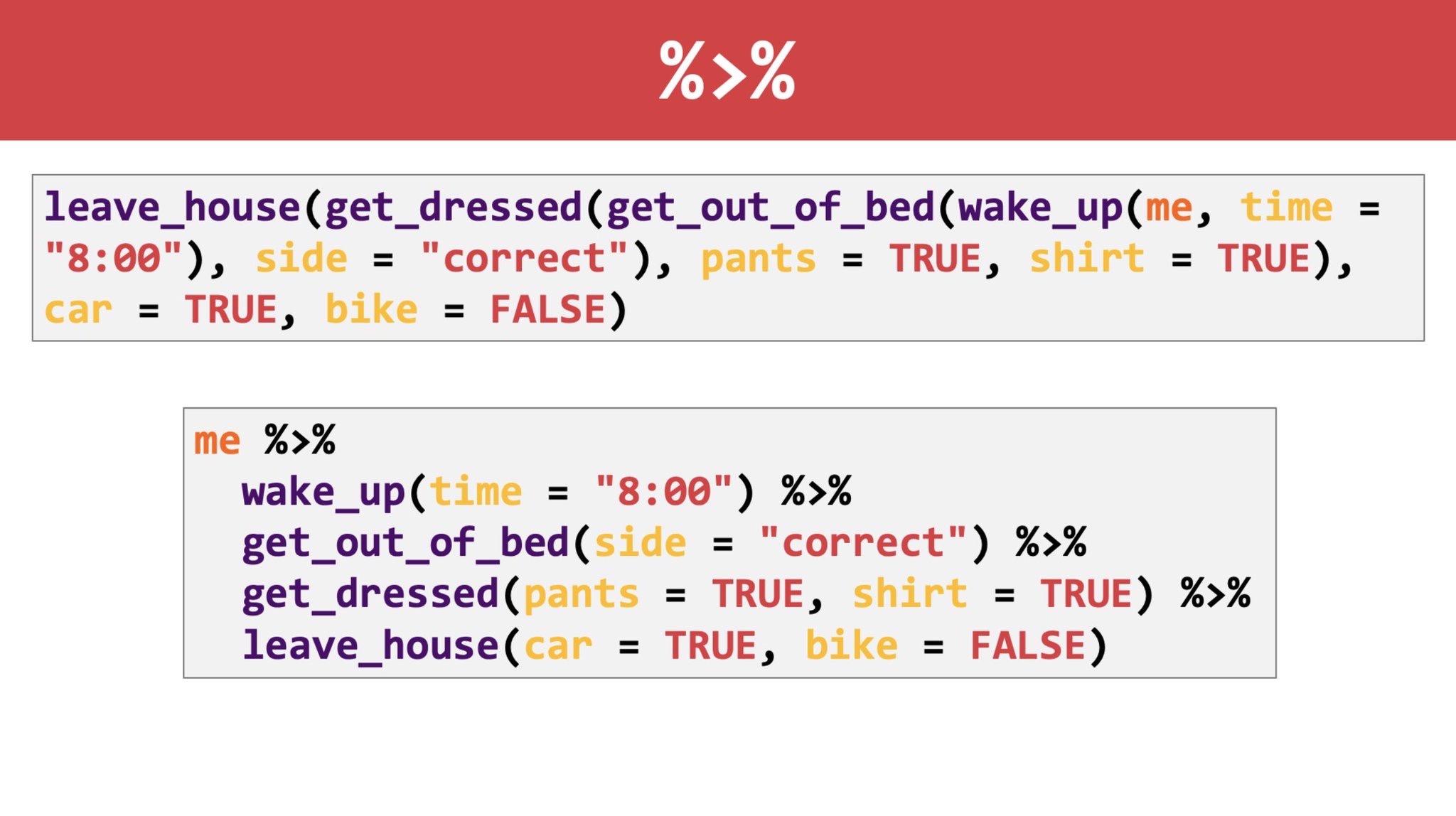
Morning Routine Pipie
20.3 The workflow:
- Wrangle your data with dplyr first
- Separate steps with
|>
- Separate steps with
- Pipe
|>your data into a plot/analysis
20.4 Basic principles:
- Do one thing at a time
- Transform variables OR select variables OR filter cases
- Chain multiple operations together using the pipe
|> - Use readable object and variable names
- Subset a dataset (i.e., select variables) by name, not by “magic numbers”
- Note that you need to use the assignment operator
<-to store changes!
20.5 Tangent: Base R workflow
We are jumping right into the tidyverse way of doing things in R, instead of the base R way of doing things. Our first week was about “just enough” base R to get you started. If you feel that you want more practice here, take a look at the R intro stat videos by MarinStatsLectures.